Quickstart
The following notebook introduces iconspy’s datatypes and some of their associated methods.
Having followed through this tutorial you will be able to construct and visusalise iconspy sections.
[1]:
from pathlib import Path
import matplotlib.pyplot as plt
import cartopy.crs as ccrs
import xarray as xr
import iconspy as ispy
import cmocean.cm as cmo
Load and prepare the example data
We will load from netcdf files as tgrid which describes the model grid, and an fxgrid which contains bathymetry information.
We then have to put them in a format that iconspy can understand. For the tgrid this means calling ispy.convert_tgrid_data, and for the the fxgrid we must make sure the dimensions have the correct names.
[2]:
shared_data_path = Path("/pool/data/ICON/oes/input/r0006/")
R02B04_path = shared_data_path / "icon_grid_0036_R02B04_O"
grid_path = R02B04_path / "R2B4_ocean-grid.nc"
fx_path = R02B04_path / "R2B4L40_fx.nc"

ds_tgrid = xr.open_dataset(grid_path)  # horizontal grid information
ds_fx = xr.open_dataset(fx_path)  # Contains bathymetry etc.

# Put datasets into the iconspy format
ds_IsD = ispy.convert_tgrid_data(ds_tgrid)

ds_fx = ds_fx.rename(
    {
        "ncells": "cell",
        "ncells_2": "edge",
        "ncells_3": "vertex",
    }
)
Define the stations we want to connect
To define a section we need two or more points to connect. Typically we have a rough idea of where we want these points to be, and we would like to choose the model grid points closest to these coordinates. Sometimes we have a desire for one of the points to be on land.
In the below we will define a section near Fram Strait, stretching from a point on Greenland to a point offshore.
[3]:
def setup_plot_area(ds_IsD):
    Slat, Nlat = -20, 20
    Wlon, Elon = -60, 0

    edges_in_region = ds_IsD["edge"].where(
        (ds_IsD["elon"] > Wlon) * (ds_IsD["elon"] < Elon) * (ds_IsD["elat"] > Slat) * (ds_IsD["elat"] < Nlat)
        , drop=True).astype("int32")


    lons = ds_IsD["vlon"].sel(vertex=ds_IsD["edge_vertices"])
    lats = ds_IsD["vlat"].sel(vertex=ds_IsD["edge_vertices"])

    fig, ax = plt.subplots(subplot_kw={"projection": ccrs.PlateCarree()})

    for edge in edges_in_region:
        ax.plot(
            lons.isel(edge=edge),
            lats.isel(edge=edge),
            color="black",
            alpha=0.2,
        )

    ax.scatter(
        ds_IsD["vlon"],
        ds_IsD["vlat"],
        s=4,
        transform=ccrs.PlateCarree(),
        color="tab:green"
    )

    ax.set_xlim(Wlon, Elon)
    ax.set_ylim(Slat, Nlat)
    ax.set_aspect("equal")

    ax.coastlines()
    ax.grid(False)
    return fig, ax
[4]:
# Put in the approximate coordinates of the points we want
# Specify that we want the George Town point to be on the boundary
target_GeorgeTown = ispy.TargetStation("George Town", -59, 6, boundary=True)
target_offshore = ispy.TargetStation("Offshore", -35, 15, boundary=False)
target_Natal = ispy.TargetStation("Natal", -35, -5, boundary=True)

# Visualise the points
fig, ax = setup_plot_area(ds_IsD)
target_GeorgeTown.plot(ax=ax, gridlines=False)
target_offshore.plot(ax=ax, gridlines=False)
target_Natal.plot(ax=ax, gridlines=False)
gl = ax.gridlines()
gl.xlines, gl.ylines = False, False
ax.grid(visible=False)
ax.legend(loc=2)
[4]:
<matplotlib.legend.Legend at 0x7f3b77288250>
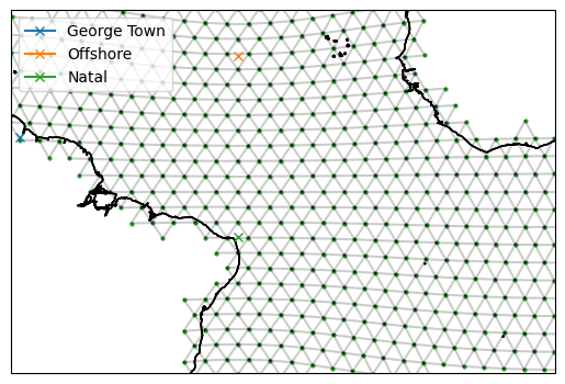
The map shows the approximate location of the points we want to join. We can now find the model grid points nearest to them and plot them.
[5]:
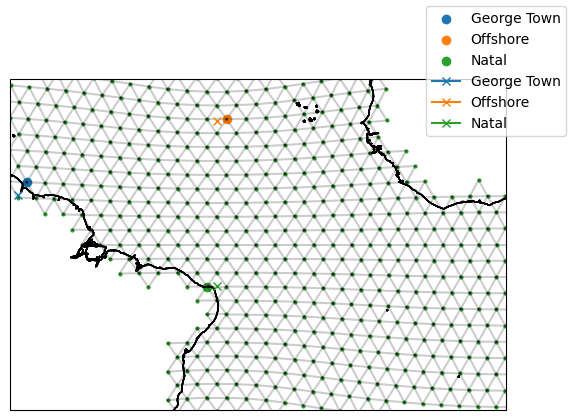
# Convert the target stations to model stations
model_GeorgeTown = target_GeorgeTown.to_model_station(ds_IsD)
model_offshore = target_offshore.to_model_station(ds_IsD)
model_Natal = target_Natal.to_model_station(ds_IsD)

fig, ax = setup_plot_area(ds_IsD)

# Plot the model stations (circles)
model_GeorgeTown.plot(ax=ax, gridlines=False)
model_offshore.plot(ax=ax, gridlines=False)
model_Natal.plot(ax=ax, gridlines=False)

# Compare with the target station (crosses)
target_GeorgeTown.plot(ax=ax, gridlines=False)
target_offshore.plot(ax=ax, gridlines=False)
target_Natal.plot(ax=ax, gridlines=False)

fig.legend()
[5]:
<matplotlib.legend.Legend at 0x7f3b771272d0>
Connect stations to form sections
[6]:
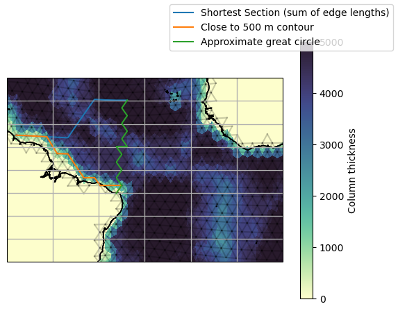
shortest = ispy.Section(
    "Shortest Section (sum of edge lengths)",
    model_GeorgeTown,
    model_offshore,
    ds_IsD,
    section_type="shortest"
)

great_circle = ispy.Section(
    "Approximate great circle",
    model_offshore,
    model_Natal,
    ds_IsD,
    section_type="great circle"
)

contour = ispy.Section(
    "Close to 500 m contour",
    model_Natal,
    model_GeorgeTown,
    ds_IsD,
    section_type="contour",
    contour_data=ds_fx["column_thick_e"],
    contour_target=500,
)

fig, ax = setup_plot_area(ds_IsD)
shortest.plot(ax=ax)
contour.plot(ax=ax)
great_circle.plot(ax=ax)

fig.legend()

cax = ax.tripcolor(
    ds_IsD["clon"],
    ds_IsD["clat"],
    ds_fx["column_thick_c"],
    vmin=0,
    vmax=5000,
    cmap=cmo.deep,
)

fig.colorbar(cax, ax=ax, label="Column thickness")
[6]:
<matplotlib.colorbar.Colorbar at 0x7f3b6cac0110>
We can get the orientation of edges along a path by running the below:
[7]:
great_circle.set_pyic_orientation_along_path(ds_IsD)
great_circle.edge_orientation
[7]:
<xarray.DataArray 'edge' (step_in_path: 13)> Size: 104B
array([ 1.,  1.,  1.,  1.,  1.,  1., -1., -1., -1., -1., -1., -1., -1.])
Coordinates:
    elon          (step_in_path) float64 104B -34.4 -34.4 ... -35.59 -35.59
    elat          (step_in_path) float64 104B 14.33 12.65 ... -2.533 -4.222
    edge          (step_in_path) int32 52B 10010 9802 9798 ... 10547 10543 10531
* step_in_path (step_in_path) int32 52B 3531 3529 3521 ... 3795 3790 3789Connect sections to form a region
[8]:
example_region = ispy.Region("Offshore of the Amazon", [shortest, great_circle, contour], ds_IsD)
/work/mh0256/m301014/iconspy/iconspy/utils.py:122: UserWarning: rename 'step_in_path_v' to 'step_in_path' does not create an index anymore. Try using swap_dims instead or use set_index after rename to create an indexed coordinate.
  edge_path_xr = edge_path_xr.rename(step_in_path_v="step_in_path")
/work/mh0256/m301014/iconspy/iconspy/utils.py:33: UserWarning: rename 'step_in_path_v' to 'step_in_path' does not create an index anymore. Try using swap_dims instead or use set_index after rename to create an indexed coordinate.
  vertex_path = vertex_path.rename(step_in_path_v="step_in_path")
[9]:
fig, ax = setup_plot_area(ds_IsD)
example_region.plot(ax=ax, gridlines=False)
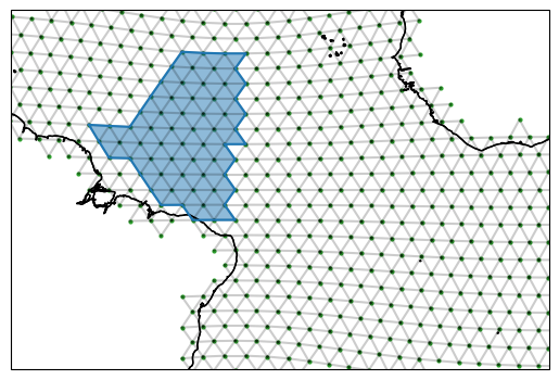
Regions have paths of edges and also edge orientations that we can use for calcualting fluxes into the region
[10]:
print(example_region.edge_circuit)
print(example_region.path_orientation)
<xarray.DataArray 'edge' (step_in_path: 32)> Size: 128B
array([ 7752, 10079, 10113, 10097, 10108,  9853, 10062, 10049, 10065, 10006,
       10010,  9802,  9798,  9782,  9789,  9872,  9866,  9864,  9878,  9882,
       10547, 10543, 10535, 10760, 10756, 10763, 10748, 10086, 10085, 10121,
       10125,  7793], dtype=int32)
Coordinates:
    elon          (step_in_path) float64 256B -50.17 -47.89 ... -49.62 -50.74
    elat          (step_in_path) float64 256B 7.166 7.053 7.848 ... 4.455 6.295
    edge          (step_in_path) int32 128B 7752 10079 10113 ... 10125 7793
    step_in_path  (step_in_path) int64 256B 1 2 3 4 5 6 7 ... 27 28 29 30 31 32
<xarray.DataArray (step_in_path: 32)> Size: 256B
array([-1.,  1., -1.,  1., -1.,  1., -1., -1.,  1., -1.,  1.,  1.,  1.,
        1.,  1.,  1., -1., -1., -1., -1., -1., -1., -1.,  1.,  1.,  1.,
       -1.,  1.,  1., -1.,  1., -1.])
Coordinates:
    elon          (step_in_path) float64 256B -50.17 -47.89 ... -49.62 -50.74
    elat          (step_in_path) float64 256B 7.166 7.053 7.848 ... 4.455 6.295
    edge          (step_in_path) int32 128B 7752 10079 10113 ... 10125 7793
  * step_in_path  (step_in_path) int64 256B 1 2 3 4 5 6 7 ... 27 28 29 30 31 32
Regions also have a list of the cells contained by them
[11]:
example_region.contained_cells
[11]:
<xarray.DataArray 'cell' (cell: 94)> Size: 376B
array([4941, 6248, 6250, 6251, 6256, 6258, 6259, 6260, 6261, 6262, 6263, 6280,
       6281, 6282, 6283, 6284, 6285, 6286, 6287, 6288, 6289, 6291, 6292, 6293,
       6294, 6295, 6297, 6299, 6300, 6301, 6302, 6303, 6305, 6390, 6426, 6435,
       6436, 6437, 6438, 6440, 6441, 6442, 6443, 6444, 6445, 6446, 6447, 6448,
       6449, 6450, 6451, 6452, 6453, 6454, 6455, 6456, 6457, 6459, 6460, 6461,
       6462, 6463, 6465, 6471, 6476, 6477, 6478, 6486, 6487, 6488, 6489, 6490,
       6491, 6492, 6493, 6494, 6495, 6496, 6497, 6498, 6499, 6500, 6501, 6731,
       6868, 6869, 6870, 6872, 6874, 6875, 6876, 6877, 6878, 6879], dtype=int32)
Coordinates:
    clon     (cell) float64 752B -50.2 -35.0 -36.19 ... -38.55 -36.18 -37.37
    clat     (cell) float64 752B 6.618 8.872 9.691 ... -0.4345 -0.4301 -2.123
* cell (cell) int32 376B 4941 6248 6250 6251 6256 ... 6876 6877 6878 6879We can also create a dataset representation of the region to be saved to a netcdf file for subsequent use.
[12]:
example_region.to_ispy_section("test.nc", dryrun=True) # set dryrun=False to actually save the file.
Output will be saved to test.nc
Not saving as dryrun=True
[12]:
<xarray.Dataset> Size: 4kB
Dimensions:           (step_in_path: 32, step_in_path_v: 33, cell: 94)
Coordinates:
    elon              (step_in_path) float64 256B -50.17 -47.89 ... -50.74
    elat              (step_in_path) float64 256B 7.166 7.053 ... 4.455 6.295
    edge              (step_in_path) int32 128B 7752 10079 10113 ... 10125 7793
  * step_in_path      (step_in_path) int64 256B 1 2 3 4 5 6 ... 28 29 30 31 32
    vlon              (step_in_path_v) float64 264B -51.3 -49.04 ... -51.3
    vlat              (step_in_path_v) float64 264B 7.224 7.106 ... 5.365 7.224
    vertex            (step_in_path_v) int32 132B 2835 2837 3618 ... 2848 2835
    clon              (cell) float64 752B -50.2 -35.0 -36.19 ... -36.18 -37.37
    clat              (cell) float64 752B 6.618 8.872 9.691 ... -0.4301 -2.123
  * cell              (cell) int32 376B 4941 6248 6250 6251 ... 6877 6878 6879
Dimensions without coordinates: step_in_path_v
Data variables:
    edge_path         (step_in_path) int32 128B 7752 10079 10113 ... 10125 7793
    vertex_path       (step_in_path_v) int32 132B 2835 2837 3618 ... 2848 2835
    path_orientation  (step_in_path) float64 256B -1.0 1.0 -1.0 ... 1.0 -1.0
    contained_cells   (cell) int32 376B 4941 6248 6250 6251 ... 6877 6878 6879
Attributes:
date: 2025-06-18 17:59:19Reconstruct sections from a region
Having produced a region we can also extract the sections that make it up. This can be useful as ordinary sections don’t have edge orientations.
[13]:
reconstructed_sections = example_region.extract_sections_from_region(ds_IsD)
[14]:
fig, ax = setup_plot_area(ds_IsD)
for section in reconstructed_sections:
    reconstructed_sections[section].plot(ax=ax, gridlines=False)
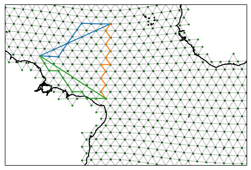
In the above we can see a funny straight line in the blue and green section. This is a bug that will be adressed in a future version. It arises from the repeating of the first vertex along the section at the end of the section. The edge paths remain unaffected though.